Variable Type

For ANOVA tests, it is necessary to have a single continuous quantitative dependent variable (DV) and a qualitative independent variable (IV) with a minimum of two levels. The IV will determine the groups that will be compared.

Independence

ANOVA tests require that the observations within each group are independent of each other, and this condition can be verified based on the study design. However, a further test, Durbin-Watson test, can be used to assess whether this assumption is satisfied or not in case needed.

Normality

ANOVA tests require the distribution of the residuals (the differences between the observed values and the predicted values) to be normal. In other words, the residuals should be normally distributed around zero and as a rule of thumb, for large sample sizes, normality is assumed to be satisfied ⁴. In this regard, there are three ways to check whether this assumption is met.

1. Via visual depiction -> using Histogram and/or Quantile-Quantile Plot (QQ Plot)
2. Via statistical testing -> using shapiro.test
   • the Null Hypothesis (\(H_{0}\)) will be data come from normal distribution, while the alternative hypothesis (\(H_{1}\)) will be data do not come from normal distribution.
   • In this scenario, having \(p-value>0.05\) will demonstrate that there is not enough evidence to reject the Null Hypothesis (\(H_{0}\)) and therefore this criterion is met.
3. Both

Equality of Variances (Homogeneity)

For this premise of the ANOVA test, the variances of the groups should be equal. 3 ways exist to check that assumption;

1. Via visual depiction -> using Histogram and/or Dot Plot and/or Scale-Location plot from plot() in R.
2. Via statistical testing -> using Levene’s test and others such as Barlett’s test and etc.
   • the Null Hypothesis (\(H_{0}\)) is variances within groups are equal, while the alternative hypothesis (\(H_{1}\)) is variances within groups are not equal.
   • In this scenario, having \(p-value>0.05\) will demonstrate that there is not enough evidence to reject the Null Hypothesis (\(H_{0}\)) and therefore this criterion is met.
3. Both

To sum up, the following figure might help which test to be used based on the specific features of the data.

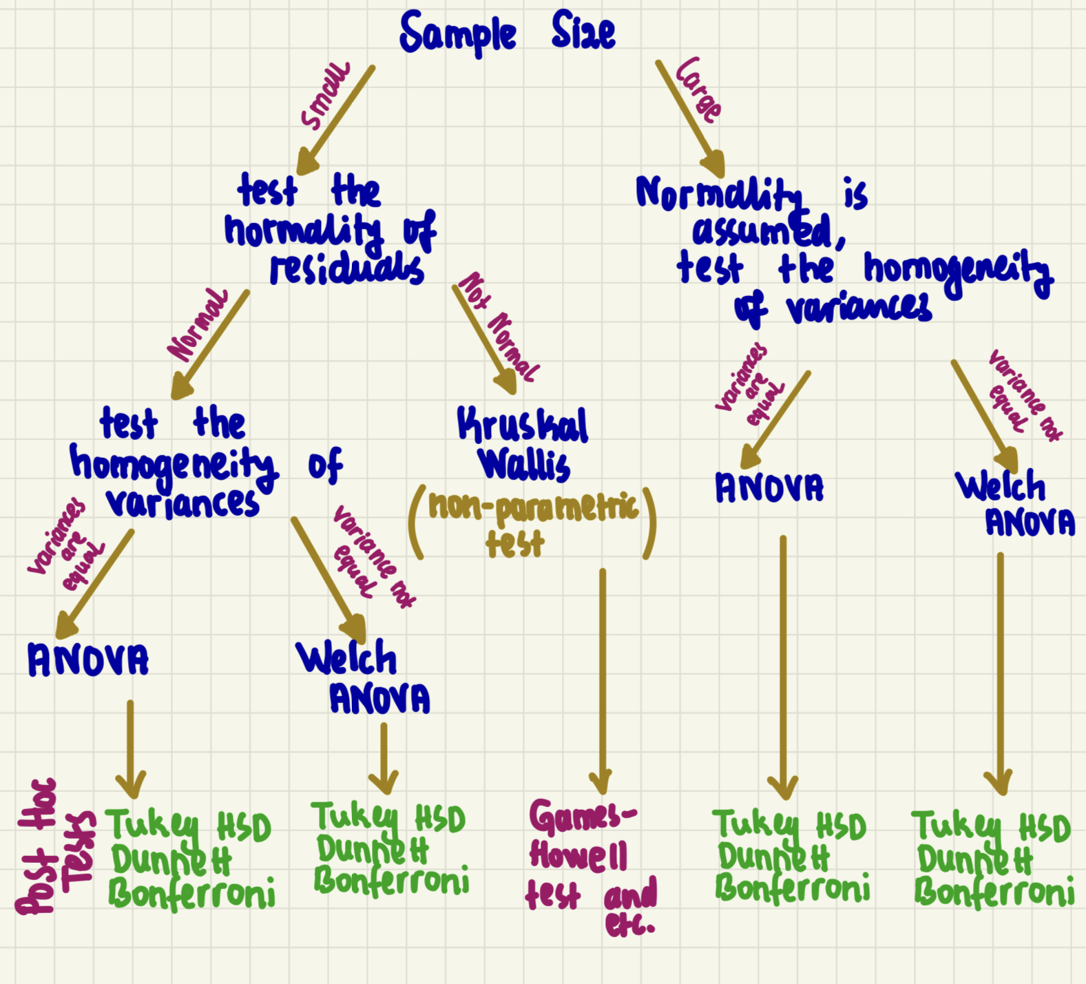
(#fig:summary_image)summary_table

Variable Type

Variable type fits to the description mentioned above. Particularly, we do have a single continuous quantitative dependent variable (DV) and a qualitative independent variable (IV) with a minimum of two levels

Independence

It can be claimed that the events are independent from the each other due to the study design we follow. One occurence is not influenced by another one.

Normality

As mentioned previously there are three ways to check normality of the ANOVA assumption. To recall them quickly, they are;

1. visually - Histogram & QQ Plot
2. statistically - via Shapiro Test
3. both

Now, let’s go over them in the following panel.

hist(full_data_1990_2020$count)

qqnorm(resid(anova_model))
qqline(resid(anova_model))

shapiro.test(full_data_1990_2020$count)

## 
##  Shapiro-Wilk normality test
## 
## data:  full_data_1990_2020$count
## W = 0.31233, p-value < 0.00000000000000022

From the initial two panels, both the histogram, showing the distribution of the number of terror events annually and the quantile-quantile (QQ) plot, showcasing the distribution of residuals, it seems that our data does not exhibit a perfect normal distribution. This observation is further confirmed by conducting the Shapiro test in the third panel, yielding a result of \(p-value<0.05\), meaning that there is enough evidence to reject the null hypothesis (\(H_{0}\)) that the data is normally distributed. However, recalling the previous discussion mentioned earlier on the normality assumption, as the sample size increases, there is a tendency to assume normality, normality will be assumed at this point.

Now, we will proceed with examining the 4^th assumption of ANOVA, which is the Equality of Variances (Homogeneity).

Equality of Variances (Homogeneity)

According to this assumption, the variances of the groups in the ANOVA test are supposed to be equal. To test that, we again have three different options;

1. visually - via Histogram & Dot Plot
2. statistically - via Levene’s Test
3. both

Now, as it has been done previously, let’s go over with these 3 options in R.

full_data_1990_2020$economic_inequality <- factor(full_data_1990_2020$economic_inequality, 
                                                  levels = c("High Inequality", "Medium Inequality", "Low Inequality"))

ggplot(full_data_1990_2020, aes(x = count, fill = economic_inequality)) +
  geom_histogram(position = "identity", alpha = 0.6) +
  labs(x = "Value", y = "Frequency") +
  ggtitle("Histograms of Values by Inequality Status") +
  facet_wrap(~ economic_inequality, nrow = 1) +
  theme(legend.position = "none")

ggplot(full_data_1990_2020, aes(x = economic_inequality, y = count)) +
  geom_point()

library(car)

leveneTest(count ~ economic_inequality, data = full_data_1990_2020)

## Levene's Test for Homogeneity of Variance (center = median)
##        Df F value      Pr(>F)    
## group   2  12.592 0.000005372 ***
##       330                        
## ---
## Signif. codes:  0 '***' 0.001 '**' 0.01 '*' 0.05 '.' 0.1 ' ' 1

Beginning with the histogram, it is evident that the variances within each group are high due to the right-skewed distribution of the number of terror events. Upon examining the dot plot, it becomes apparent that the variances within each group also exhibit a considerable variation. To statistically test this using Levene’s test in the third panel, the resulting \(p-value\) is found to be lower than 0.05, indicating sufficient evidence to reject the null hypothesis (\(H_{0}\)) that the variances are equal across groups.